Week 10 - Data Wrangling Part I

In this part of the session, we are going to learn how to use key packages and functions that enable you to conduct data cleaning in R.

By the end of this session, you should be capable of the following:

Use the functions select(), mutate(), rename(), to perform key operations on columns.
Use the functions filter(), arrange(), and distinct() to perform key operations on rows.
Understand how to group information and perform calculations on those groupings.
Understand how to pipe together functions to enable efficient data cleaning analysis.

Let’s Get Set Up

Let’s begin by ensuring your working environment is ready for today’s session. Open RStudio or Posit Cloud and complete the following tasks to set everything up.

Activity 1: Set Up Your Working Directory & R Script for this week

First, create a folder named week10 inside your course directory and set it as your working directory.

Reminder on Steps to Set Up Your Working Directory

Click:
Session → Set Working Directory → Choose Directory
Navigate to the folder you created for this course (this should be the same folder you used for previous workshops).
Create a new folder called week10 inside this directory.
Select the week10 folder and click Open.

Don’t forget to verify your working directory before we get started

You can always check your current working directory by typing in the following command in the console:

getwd()

[1] "C:/Users/0131045S/Desktop/R/rintro/activities/week10"

Next, we will create our first R script for today. We will be creating more than one. Call your first script 10-data-wrangling-p1.

Reminder on creating an R script

Go to the menu bar and select:
File → New File → R Script

This will open an untitled R script.
To save and name your script, select:

File→ Save As, then enter the name:

10-data-wrangling-p1

Click Save

Activity 2: Installing / Loading R Packages

We only need one package for data wrangling - tidyverse. But we will need to run descriptives also, so we will load in the jmv package

library(tidyverse)
library(jmv)

REMEMBER: If you encounter an error message like “Error in library(package name): there is no packaged calledpackage name”, you’ll need to install the package first by editing the following for your console:

install.packages("tidyverse") #replace "package name" with the actual package name

Activity 3: Load in your datasets

In this exercise, we will clean the Flanker Test Dataset, which was collected as part of a study investigating the effect of alcohol consumption on inhibiting incongruent responses (e.g., the flanker effect).

The dataset includes responses from 50 participants, who provided information on their age, gender, and mean Neuroticism scores. Additionally, participants were split into two conditions:

Control (no alcohol)
Experimental (high alcohol)

Download the Dataset

Download the file flanker.csv onto your computer and move it to your week10 folder.

Load the Dataset into R

Once you have downloaded the file, load it into R and save it as a dataframe named df_flanker_raw:

Tip

df_flanker_raw <- read.csv("flanker.csv")

Activity 4: Inspect your Data set

The first step after importing a dataset is to check it to ensure that we have imported the correct data. We can do this using the head() function:

head(df_flanker_raw)

  Private.ID Experiment.Status aGe     status nero3 net2  X X.1 neuro5
1          1           preview  32 experiment     2    2 NA  NA      5
2          2           preview  37    control     3    2 NA  NA      3
3          3           preview  28 experiment     4    3 NA  NA      2
4          4           preview  30    control     2    3 NA  NA      4
5          5           preview  28 experiment     2    2 NA  NA      2
6          6           preview  33    control     3    3 NA  NA      2
  nationality wlanker_congruent flanker_incongruent Participant.OS
1        Male               643                 607     Windows 10
2      Female               545                 625     Windows 10
3  Non-Binary               629                 556     Windows 10
4        Male               616                 617     Windows 10
5      Female               794                 752     Windows 10
6  Non-Binary               629                 529     Windows 10
  Local.Timestamp neuro1 neuro4
1        1.71E+12      3      4
2        1.71E+12      3      3
3        1.71E+12      4      4
4        1.71E+12      2      3
5        1.71E+12      4      3
6        1.71E+12      2      3

What if I want to view the entire dataset?

You can click on the dataset in the Environment page to view it

Ouch! Now that is a dataset only a parent could love. Here’s what each column tells us about each participant:

Column	Description
Private.ID	Experiment ID.
Experiment.Status	Indicates whether the study was published (live) or not (preview) for each participant.
aGe	Participant’s age.
status	Indicates whether the participant was in the experiment or control group.
nero3	Participant’s score on the 3rd item from a Neuroticism scale.
net2	Participant’s score on the 2nd item from a Neuroticism scale.
X	An empty column. NA values indicate missing data (Not Available).
X.1	Another empty column.
neuro5	Participant’s score on the 5th item from a Neuroticism scale.
nationality	Participant’s gender.
wlanker_congruent	Participant’s average reaction time (ms) on the flanker task when the stimulus/flanker direction was congruent. (An unfortunately suggestive misspelling!)
flanker_incongruent	Participant’s average reaction time (ms) on the flanker task when the stimulus/flanker direction was incongruent.
Participant.OS	The operating system the participant used to take the survey.
Local.Timestamp	Timestamp indicating when participants took part in the study.
neuro1	Participant’s score on the 1st item from a Neuroticism scale.
neuro4	Participant’s score on the 4th item from a Neuroticism scale.

Issues in the Dataset:

Several issues are evident in this dataset:

Unnecessary columns: Variables like "Local.Timestamp" and "Participant.OS" are not needed for our analysis.
Misspelled or inconsistent column names: Columns such as "Participant.Private.ID", "wlanker_congruent", and "nero3" are awkwardly named, misspelled, or inconsistent.
Disorganized column order: The dataset is not structured optimally—important variables (e.g., Neuroticism items) are scattered throughout.
Incomplete scoring: We want to analyse participants’ total Neuroticism scores, but only have individual item scores.
Incorrect information: The "nationality" column actually contains participants’ gender.
Unexpected participant count: The dataset reports 60 participants instead of the expected 50.
Presence of preview data: The dataset contains responses from both preview and live study phases. Preview data needs to be removed.

Key Functions That Will Help You Clean Most Datasets

The following functions, all from the tidyverse package, will help us clean the df_flanker_raw dataset. Each function serves a unique purpose:

Function	Description
`select()`	Include or exclude certain variables (columns)
`filter()`	Include or exclude certain observations (rows)
`mutate()`	Create new variables (columns)
`arrange()`	Change the order of rows
`disinct()`	Select unique observations (rows) / identify duplicate values.
`rename()`	Rename variables (columns)

We will use each of these functions in this chapter to clean the df_flanker_raw dataset—so you’ll get plenty of practice!

Activity 5: Renaming Columns with `rename()`

When cleaning a dataset, one of the first things you should do is identify the columns that you need for your analysis or that contain important information.

In our case, these columns include the participant’s ID (Private.ID), whether they completed the study or a preview (Experiment.Status), whether they were in the experimental or control group (status), their Neuroticism scores (neuro1, net2, nero3, neuro4, neuro5), demographic information (aGe, nationality), and their reaction times on the flanker trials (wlanker_congruent & flanker_incongruent).

The first step is to rename any awkward or inconsistent column names to make them easier to work with—because good grief, these names are ugly!

Luckily, we can rename these columns using the rename() function.

The syntax for this function is slightly counterintuitive in its order, as it follows this structure:

rename(dataframe, newcolumnane = oldcolumnname)

For our dataset, we will rename the relevant columns:

df_flanker_renamed <- rename(df_flanker_raw,
                             ID = Private.ID,
                             neuro2 = net2,
                             neuro3 = nero3,
                             flanker_congruent = wlanker_congruent,
                             age = aGe,
                             gender = nationality,
                             group = status,
                             experiment_status = Experiment.Status)


head(df_flanker_renamed)

  ID experiment_status age      group neuro3 neuro2  X X.1 neuro5     gender
1  1           preview  32 experiment      2      2 NA  NA      5       Male
2  2           preview  37    control      3      2 NA  NA      3     Female
3  3           preview  28 experiment      4      3 NA  NA      2 Non-Binary
4  4           preview  30    control      2      3 NA  NA      4       Male
5  5           preview  28 experiment      2      2 NA  NA      2     Female
6  6           preview  33    control      3      3 NA  NA      2 Non-Binary
  flanker_congruent flanker_incongruent Participant.OS Local.Timestamp neuro1
1               643                 607     Windows 10        1.71E+12      3
2               545                 625     Windows 10        1.71E+12      3
3               629                 556     Windows 10        1.71E+12      4
4               616                 617     Windows 10        1.71E+12      2
5               794                 752     Windows 10        1.71E+12      4
6               629                 529     Windows 10        1.71E+12      2
  neuro4
1      4
2      3
3      4
4      3
5      3
6      3

We can also verify the updated column names in our dataframe by using the colnames() function, which will print only the names of the columns in our dataframe:

colnames(df_flanker_renamed)

 [1] "ID"                  "experiment_status"   "age"                
 [4] "group"               "neuro3"              "neuro2"             
 [7] "X"                   "X.1"                 "neuro5"             
[10] "gender"              "flanker_congruent"   "flanker_incongruent"
[13] "Participant.OS"      "Local.Timestamp"     "neuro1"             
[16] "neuro4"

Either way, we now have clearer and more consistent column names for the data we need.

Next, let’s remove the columns that we do not need for our analysis.

Activity 6: Selecting columns with select()

We can use the select() function to extract only the columns we need from a dataframe. The syntax for this function is:

The syntax for this function is: select(dataframe, c(col1name, col2name, col3name))

For this exercise, we will select only the relevant columns and store them in a new dataframe called df_flanker_selected:

df_flanker_selected <- select(df_flanker_renamed, c(ID,
                                                experiment_status,
                                                group,
                                                age,
                                                gender,
                                                flanker_congruent,
                                                flanker_incongruent,
                                                neuro1,
                                                neuro2,
                                                neuro3,
                                                neuro4,
                                                neuro5))

head(df_flanker_selected)

  ID experiment_status      group age     gender flanker_congruent
1  1           preview experiment  32       Male               643
2  2           preview    control  37     Female               545
3  3           preview experiment  28 Non-Binary               629
4  4           preview    control  30       Male               616
5  5           preview experiment  28     Female               794
6  6           preview    control  33 Non-Binary               629
  flanker_incongruent neuro1 neuro2 neuro3 neuro4 neuro5
1                 607      3      2      2      4      5
2                 625      3      2      3      3      3
3                 556      4      3      4      4      2
4                 617      2      3      2      3      4
5                 752      4      2      2      3      2
6                 529      2      3      3      3      2

That looks much cleaner already!

You may have noticed that the order of columns in df_flanker_selected matches the order in which they were listed inside select(). This is a useful feature that allows us to easily reorder our dataframe.

Now, I want you to modify df_flanker_selected so that our dependent variables (flanker_congruent and flanker_incongruent) appear immediately after the group column, before the other variables. The output should look like this:

  ID experiment_status      group flanker_congruent flanker_incongruent age
1  1           preview experiment               643                 607  32
2  2           preview    control               545                 625  37
3  3           preview experiment               629                 556  28
4  4           preview    control               616                 617  30
5  5           preview experiment               794                 752  28
6  6           preview    control               629                 529  33
      gender neuro1 neuro2 neuro3 neuro4 neuro5
1       Male      3      2      2      4      5
2     Female      3      2      3      3      3
3 Non-Binary      4      3      4      4      2
4       Male      2      3      2      3      4
5     Female      4      2      2      3      2
6 Non-Binary      2      3      3      3      2

What if I have lots of columns, do I have to type everything out?

When working with large datasets, manually specifying every column can be tedious. Fortunately, select() has several shortcuts that make life easier.

Removing Columns with `-` Operator

If you want to exclude specific columns instead of selecting them, use the - operator before the column name.

For example, to remove the gender column:

df_flanker_remove_gender <- select(df_flanker_selected, -c(gender))

colnames(df_flanker_remove_gender)

 [1] "ID"                  "experiment_status"   "group"              
 [4] "flanker_congruent"   "flanker_incongruent" "age"                
 [7] "neuro1"              "neuro2"              "neuro3"             
[10] "neuro4"              "neuro5"

And voilà—gender is gone!

Similarly, you can remove multiple columns

df_flanker_remove_demographics <- select(df_flanker_selected, -c(gender, age))

colnames(df_flanker_remove_demographics)

 [1] "ID"                  "experiment_status"   "group"              
 [4] "flanker_congruent"   "flanker_incongruent" "neuro1"             
 [7] "neuro2"              "neuro3"              "neuro4"             
[10] "neuro5"

Selecting Consecutive Columns with `:`

The : operator allows you to select a range of columns that are next to each other.

For example, to keep only the ID column and the Neuroticism scale items:

df_flanker_select_simultaneous <- select(df_flanker_selected, c(ID, neuro1:neuro5))

head(df_flanker_select_simultaneous)

  ID neuro1 neuro2 neuro3 neuro4 neuro5
1  1      3      2      2      4      5
2  2      3      2      3      3      3
3  3      4      3      4      4      2
4  4      2      3      2      3      4
5  5      4      2      2      3      2
6  6      2      3      3      3      2

Combining `-` (Remove) and `:` (Select a Range)

You can combine both techniques to remove a consecutive range of columns.

For example, to remove ID, age, and all Neuroticism items (neuro1 to neuro5):

df_flanker_unselect_simultaneous <- select(df_flanker_selected, -c(ID, age, neuro1:neuro5))

head(df_flanker_unselect_simultaneous)

  experiment_status      group flanker_congruent flanker_incongruent     gender
1           preview experiment               643                 607       Male
2           preview    control               545                 625     Female
3           preview experiment               629                 556 Non-Binary
4           preview    control               616                 617       Male
5           preview experiment               794                 752     Female
6           preview    control               629                 529 Non-Binary

Now, ID, age, and all Neuroticism-related columns are gone!

Activity 7: Creating New Columns using `mutate()`

So far, we have removed unnecessary columns and renamed the remaining ones. However, one key variable is missing.

At the moment, we have individual item scores for Neuroticism (neuro1 to neuro5). Since we’re not conducting a reliability or factor analysis, we need a total Neuroticism score for each participant.

The mutate() function allows us to create new columns by applying operations to existing ones.

The syntax for this function is:

mutate(df, new_column_name = instructions on what to do with current columns)

Let’s use mutate() to create a new column called neuroticism_total, which sums the five Neuroticism items:

df_flanker_mutated <- mutate(df_flanker_selected, 
                    neuroticism_total = neuro1 + neuro2 + neuro3 + neuro4 + neuro5)
                    #new_col_name = operation on current columns

head(df_flanker_mutated)

  ID experiment_status      group flanker_congruent flanker_incongruent age
1  1           preview experiment               643                 607  32
2  2           preview    control               545                 625  37
3  3           preview experiment               629                 556  28
4  4           preview    control               616                 617  30
5  5           preview experiment               794                 752  28
6  6           preview    control               629                 529  33
      gender neuro1 neuro2 neuro3 neuro4 neuro5 neuroticism_total
1       Male      3      2      2      4      5                16
2     Female      3      2      3      3      3                14
3 Non-Binary      4      3      4      4      2                17
4       Male      2      3      2      3      4                14
5     Female      4      2      2      3      2                13
6 Non-Binary      2      3      3      3      2                13

df_flanker_mutated$neuroticism_total

 [1] 16 14 17 14 13 13 13 13 16 14 13 16 17 12 14 14 13 15 13 17 16 16 16 16 13
[26] 15 15 14 16 11 16 18 17 14 13 13 13 14 14 15 17 17 18 19 15 15 15 16 13 20
[51] 20  9 13 14 15 15 14 11 15 14 16 13

What if I want to calculate the mean?

If we wanted to calculate the mean of these items (rather than the total score), we need to ensure that R calculates the mean per participant (row-wise) rather than across the entire dataset.

To do this, we use the rowMeans() function, which calculates the mean for each row (i.e., for each participant).

Since rowMeans() requires us to specify which columns to use, we must first select the relevant columns inside mutate().

Let’s save this new variable as neuroticism_mean:

df_flanker_mutated_average <- mutate(df_flanker_mutated, 
                    #we use `select()` to pick the columns we want
                    neuroticism_mean = rowMeans(select(df_flanker_mutated, 
                                                    c(neuro1, neuro2, neuro3,
                                                      neuro4, neuro5))))
                    

head(df_flanker_mutated_average)

  ID experiment_status      group flanker_congruent flanker_incongruent age
1  1           preview experiment               643                 607  32
2  2           preview    control               545                 625  37
3  3           preview experiment               629                 556  28
4  4           preview    control               616                 617  30
5  5           preview experiment               794                 752  28
6  6           preview    control               629                 529  33
      gender neuro1 neuro2 neuro3 neuro4 neuro5 neuroticism_total
1       Male      3      2      2      4      5                16
2     Female      3      2      3      3      3                14
3 Non-Binary      4      3      4      4      2                17
4       Male      2      3      2      3      4                14
5     Female      4      2      2      3      2                13
6 Non-Binary      2      3      3      3      2                13
  neuroticism_mean
1              3.2
2              2.8
3              3.4
4              2.8
5              2.6
6              2.6

Using `.keep` to Remove Unnecessary Columns

If we no longer need the original Neuroticism item scores (neuro1 to neuro5), we can automatically remove them by using the .keep argument inside mutate().

The .keep argument controls what happens to the original columns:

.keep = "all" (default) → Keeps all original columns.
.keep = "unused" → Removes the columns used in the calculation.
.keep = "none" → Removes all columns except the newly created one.

Since we only need the total score, let’s use .keep = "unused"

df_flanker_mutated_exclusive <- mutate(df_flanker_selected, 
                    neuroticism_total = neuro1 + neuro2 + neuro3 + neuro4 + neuro5,
                    .keep = "unused")

head(df_flanker_mutated_exclusive)

  ID experiment_status      group flanker_congruent flanker_incongruent age
1  1           preview experiment               643                 607  32
2  2           preview    control               545                 625  37
3  3           preview experiment               629                 556  28
4  4           preview    control               616                 617  30
5  5           preview experiment               794                 752  28
6  6           preview    control               629                 529  33
      gender neuroticism_total
1       Male                16
2     Female                14
3 Non-Binary                17
4       Male                14
5     Female                13
6 Non-Binary                13

This means the original columns (neuro1 to neuro5) have been removed, leaving only the new total score.

Since we no longer need the individual items, we will use this new dataframe moving forward.

Checking in on our data

We’ve made significant progress in cleaning our dataset. So far, we have:

Removed unnecessary columns
Fixed column names and ordering
Created new columns for our analysis.
Corrected errors in existing columns.

Our dataset is almost ready for analysis!

However, there are still extra participants in our dataset that we need to remove. We expect 50 participants, but if we check the number of rows, we see that there are actually 62 participants.

nrow(df_flanker_mutated_exclusive)

[1] 62

So, where did these extra 12 participants come from?

If you look at the experiment_status column in our dataset, you’ll notice that it contains both preview and live data. We can use the table() function to count how many participants contributed to each category:

table(df_flanker_mutated_exclusive$experiment_status)


   live preview 
     52      10

The output tells us that 10 of the 12 extra participants are from preview data. However, we still have two additional participants who completed the study under live conditions.

Before proceeding, we need to investigate why we have these extra participants in the live condition.

Activity 8 - Removing Duplicates using `distinct()`

Why Do We Have Extra Participants?

In the previous step, we discovered that our dataset contains 12 extra participants instead of the expected 50. While we identified that 10 of these participants were part of the preview phase, there are still two additional participants that we need to investigate.

One possible explanation is that some participants data were accidently duplicated when downloading the dataset.

Step 1: Identifying Duplicate Rows

The duplicated() function checks whether each row in a dataframe is an exact duplicate of a previous row.

duplicated(df_flanker_mutated_exclusive)

 [1] FALSE FALSE FALSE FALSE FALSE FALSE FALSE FALSE FALSE FALSE FALSE FALSE
[13] FALSE FALSE FALSE FALSE FALSE FALSE FALSE FALSE FALSE FALSE FALSE FALSE
[25] FALSE FALSE FALSE FALSE FALSE FALSE FALSE FALSE FALSE FALSE FALSE FALSE
[37] FALSE FALSE FALSE FALSE FALSE FALSE FALSE FALSE FALSE FALSE FALSE FALSE
[49]  TRUE FALSE FALSE FALSE FALSE FALSE FALSE FALSE FALSE FALSE FALSE FALSE
[61] FALSE  TRUE

The function returns a logical vector of TRUE and FALSE values:

TRUE means the row is a duplicate.
FALSE means the row is unique.

Each TRUE or FALSE corresponds to a row in the dataframe.

If we want to extract and see the duplicated rows, we can follow the syntax we discussed in Chapter 3 about extracting values from a dataframe: dataframe[rows_we_want, columns_we_want]

df_flanker_mutated_exclusive[duplicated(df_flanker_mutated_exclusive), ]

   ID experiment_status      group flanker_congruent flanker_incongruent age
49 11              live experiment               753                 574  25
62 11              live experiment               753                 574  25
   gender neuroticism_total
49 Female                13
62 Female                13

From this output, we see that the participant with ID = 11 has duplicate rows.

Step 2: Removing Duplicate Rows with `distinct()`

Now that we have identified the duplicated participant, we need to remove them.

The distinct() function removes any duplicate rows, ensuring that only unique records remain.

To remove these values we can use the distinct() function. This function takes in a data frame or a column and only keeps the rows that are unique.

df_flanker_distinct <- distinct(df_flanker_mutated_exclusive)

To confirm that the duplicate has been removed, we can check the number of participants in each study phase again using table():

table(df_flanker_distinct$experiment_status)


   live preview 
     50      10

It looks like we have. We can also double-check this by calling the duplicated() function again to see if any values return as TRUE

duplicated(df_flanker_distinct)

 [1] FALSE FALSE FALSE FALSE FALSE FALSE FALSE FALSE FALSE FALSE FALSE FALSE
[13] FALSE FALSE FALSE FALSE FALSE FALSE FALSE FALSE FALSE FALSE FALSE FALSE
[25] FALSE FALSE FALSE FALSE FALSE FALSE FALSE FALSE FALSE FALSE FALSE FALSE
[37] FALSE FALSE FALSE FALSE FALSE FALSE FALSE FALSE FALSE FALSE FALSE FALSE
[49] FALSE FALSE FALSE FALSE FALSE FALSE FALSE FALSE FALSE FALSE FALSE FALSE

All values are FALSE—this confirms that our dataset no longer contains duplicates.

Now that we have removed duplicate participants, our next step is to clean up the preview data from our dataset.

Activity 9 - Selecting Rows using `filter()`

Removing Rows Using `filter()`

The filter() function allows us to select rows that meet specific conditions while filtering out those that do not. Its syntax follows this structure: filter(dataframe, condition), where the condition specifies which rows to retain.

In our dataset, the experiment_status column tells us whether a participant was part of the live or preview study. We only want to keep participants who completed the live version of the study and remove all preview data.

We can do this using filter():

df_flanker_filtered <- filter(df_flanker_distinct, experiment_status == "live")

The condition experiment_status == "live" instructs R to keep only rows where the experiment_status column is "live".

To confirm that we have successfully removed all preview participants, we can use the table() function:

table(df_flanker_filtered$experiment_status)


live 
  50

The output now only contains "live", meaning that all "preview" data has been successfully removed.

What if I want to tell R what not to select?

We can also exclude specific rows using filter().

For example, instead of specifying that we want only "live" rows, we could remove "preview" rows using !=, which means “not equal to”:

df_filter_neg <- filter(df_flanker_distinct, experiment_status != "preview")

table(df_filter_neg$experiment_status)


live 
  50

Here, != tells R to keep everything except "preview".

This is especially useful when a column contains multiple values, and it’s easier to exclude certain ones rather than specify every value you want to keep.

Since we have removed the preview scores from our status column, do we actually need it anymore? Probably not as it won’t be used in our final analysis. So let’s remove it using the select() function and - operator.

df_flanker_filtered <- select(df_flanker_filtered, -c(experiment_status))

head(df_flanker_filtered)

  ID      group flanker_congruent flanker_incongruent age     gender
1 11 experiment               753                 574  25     Female
2 12    control               655                 719  25 Non-Binary
3 13 experiment               747                 680  31       Male
4 14    control               554                 509  31     Female
5 15 experiment               567                 588  28 Non-Binary
6 16    control               544                 505  26       Male
  neuroticism_total
1                13
2                16
3                17
4                12
5                14
6                14

Removing Rows Using Multiple Conditions with `filter()`

We can also use filter() to check whether rows meet several conditions at the same time. For example, let’s look at our columns flanker_congruent and flanker_incongruent, which contains participants reaction times (ms).

When cleaning reaction time (RT) data, it’s common to remove extreme values that are likely due to accidental premature responses or inattentiveness. The choice of cutoff points depends on the nature of your experiment and the typical response range, but for the sake of our analysis, let’s go with the following:

Very fast responses (e.g., under 100 ms) might indicate that a participant anticipated the stimulus or accidentally pressed a button.
Very slow responses (e.g., over 2000 ms) might suggest that a participant was distracted or inattentive

In this case, we want to remove any participant’s data who scored too fast or too slow on either flanker_congruent OR flanker_incongruent.

Step 1: Checking for Extreme Values

Before filtering, let’s first check if any participants fall outside our thresholds. We will start by inspecting the flanker_congruent column.

sort(df_flanker_filtered$flanker_congruent)

 [1]  50  60 505 514 525 525 538 542 544 544 553 554 555 561 565 567 568 574 575
[20] 588 592 598 613 627 628 638 640 651 655 676 690 694 698 705 707 725 743 744
[39] 747 751 753 763 768 776 777 787 789 789 797 800

What are we doing here?

The sort() function sorts the values from smallest to largest, allowing us to quickly see any extreme values.

What do we find?

Two participants have reaction times under 100 ms.
One participant has a reaction time of 2000 ms.

Next, let’s check the flanker_incongruent column.

sort(df_flanker_filtered$flanker_incongruent)

 [1]  505  509  516  519  529  535  536  540  542  549  558  564  574  580  582
[16]  585  588  595  601  607  611  613  629  647  650  658  665  672  680  682
[31]  684  694  707  711  715  716  719  720  727  734  734  741  747  750  756
[46]  766  772  785  793 3000

What do we find?

No participants have reaction times under 100 ms.
One participant has a reaction time of 3000 ms, which exceeds our 2000 ms threshold.

Step 2: Removing Extreme Values Using `filter()`

Now that we know which values to exclude, we will use filter() to remove all participants who have:

RTs below 100 ms in either flanker_congruent OR flanker_incongruent.
RTs above 2000 ms in either flanker_congruent OR flanker_incongruent

df_flanker_filtered_ms <- filter(df_flanker_filtered,
                                 flanker_congruent >= 100 & flanker_congruent <= 2000,
                                 flanker_incongruent >= 100 & flanker_incongruent <= 2000)

What the hell is happening here? Let’s break down the code

flanker_congruent >= 100 & flanker_congruent <= 2000
- Keep rows where flanker_congruent is at least 100 AND at most 2000.

flanker_incongruent >= 100 & flanker_incongruent <= 2000
- Keep rows where flanker_incongruent is at least 100 AND at most 2000.

Step 3: Confirming Data Changes

Now let’s check how many participants remain after filtering.

nrow(df_flanker_filtered_ms)

[1] 47

We can see that we have three fewer participants. But in this case, although our sample is smaller, the quality of our data is now more consistent.

Activity 10: Save your Clean Data

There we have it! We have successfully cleaned our first data frame in R. Well done.

Now that we have successfully cleaned the dataset, let’s rename it and export it so that we can use it in future analyses.

df_flanker_clean <- df_flanker_filtered

write.csv(df_flanker_clean, "df_clean.csv", row.names = F)

Final Activity: Save Reckless Ryan

On the week I was supposed to submit my master’s dissertation, I realised I had made major errors while cleaning my dataset.

Some rows should never have been included, some variables had the wrong names, some columns were irrelevant, some participants were duplicated, and some values were clearly impossible.

If I submitted the dataset like this, a lot of my results and conclusions would be false.

I do not have time to clean the data by hand.
I need to use R to rescue the dataset.

Study background

This study investigated whether walking for 10 minutes in a natural environment versus an urban environment influenced cognitive reasoning.

Participants completed 8 belief-bias syllogisms after the walk.
Higher scores indicate better reasoning performance.

Participants also completed:

a 3-item Cognitive Reflection Test (CRT)
a verbal fluency task

These are included as control variables.

Your task

Load the dataset and clean it into a new dataframe called:

df_clean

The raw dataset is called:

df_masters_raw

Use only functions and ideas from this week’s worksheet where possible:

rename()
select()
mutate()
distinct()
filter()
arrange()

What needs to be fixed

1. Rename key columns

Rename the following variables:

Participant.no → id
Study.Status → study_status
AgeYears → age
conditoin → condition
country → gender
fluency_scoree → verbal_fluency
crt_one → crt1
CRt2 → crt2
syllogism_1 → syll1
identify and fix the other syllogism items in a consistent format (e.g. syll2, syll3, etc)

2. Keep only relevant columns

Keep only:

id, study_status, age, gender, condition,
syll1, syll2, syll3, syll4, syll5, syll6, syll7, syll8,
crt1, crt2, crt3, verbal_fluency

3. Create new variables

Using mutate(), create:

belief_bias_total = sum of the 8 syllogism items
crt_total = sum of the 3 CRT items
Use mutate to remove the individual CRT items and 8 belief bias syllogisms.

4. Reorder columns

Reorder the dataset so it follows this structure:

id, study_status, age, gender, condition,
crt1, crt2, crt3, verbal_fluency,
belief_bias_total, crt_total

5. Remove preview rows

Only keep participants who completed the study.

6. Remove duplicates

Remove any duplicated rows.

7. Remove impossible values

Remove participants who meet any of the following:

age below 18 or above 100
verbal_fluency below 0 or above 60

8. Arrange the dataset

Sort the cleaned dataset by id from smallest to largest.

9. Save the cleaned dataset

Save your final dataset as:

masters_belief_bias_clean.csv

Final check

If you cleaned the dataset correctly, it should contain:

134 rows (participants)
7 columns (variables)

And the first 10 rows should look like this:

     id age gender condition verbal_fluency belief_bias_total crt_total
1  1001  45   Male     urban             19                 6         1
2  1002  33   Male     urban             10                 6         3
3  1003  43 Female     urban             43                 6         2
4  1004  39 Female     urban             25                 4         1
5  1006  29 Female     urban             12                 3         2
6  1007  32 Female     urban             29                 6         2
7  1008  26   Male     urban             34                 7         3
8  1009  22 Female     urban             34                 4         1
9  1010  23 Female     urban             38                 7         1
10 1012  21   Male     urban             22                 3         2

Run descriptive statistics and an independent sample t-test to assess whether you get the same results as me.

options(scipen = 999)

library(jtools)

descriptives(data = df_clean,
             vars = c("verbal_fluency", "belief_bias_total", "crt_total"),
             splitBy = "condition",
             desc = "rows")


 DESCRIPTIVES

 Descriptives                                                                                                     
 ──────────────────────────────────────────────────────────────────────────────────────────────────────────────── 
                        condition    N     Missing    Mean         Median       SD           Minimum    Maximum   
 ──────────────────────────────────────────────────────────────────────────────────────────────────────────────── 
   verbal_fluency       natural      68          0    27.470588    27.000000    7.5319629          7         44   
                        urban        66          0    27.939394    29.000000    7.4871763          6         43   
   belief_bias_total    natural      68          0     5.661765     6.000000    1.5023394          1          8   
                        urban        66          0     4.651515     5.000000    1.3184189          2          7   
   crt_total            natural      68          0     1.500000     2.000000    0.9060328         -1          3   
                        urban        66          0     1.696970     2.000000    0.9441267          0          4   
 ────────────────────────────────────────────────────────────────────────────────────────────────────────────────

ggplot(df_clean, aes(x = condition, y = belief_bias_total, fill = condition)) +
  geom_violin() +
  geom_boxplot() +
  stat_summary(fun = mean, geom = "point", size = 4, shape = 18) +
  labs(
    title = "Belief-bias scores by environment condition",
    x = "Condition",
    y = "Belief-bias total"
  ) +
  theme_apa()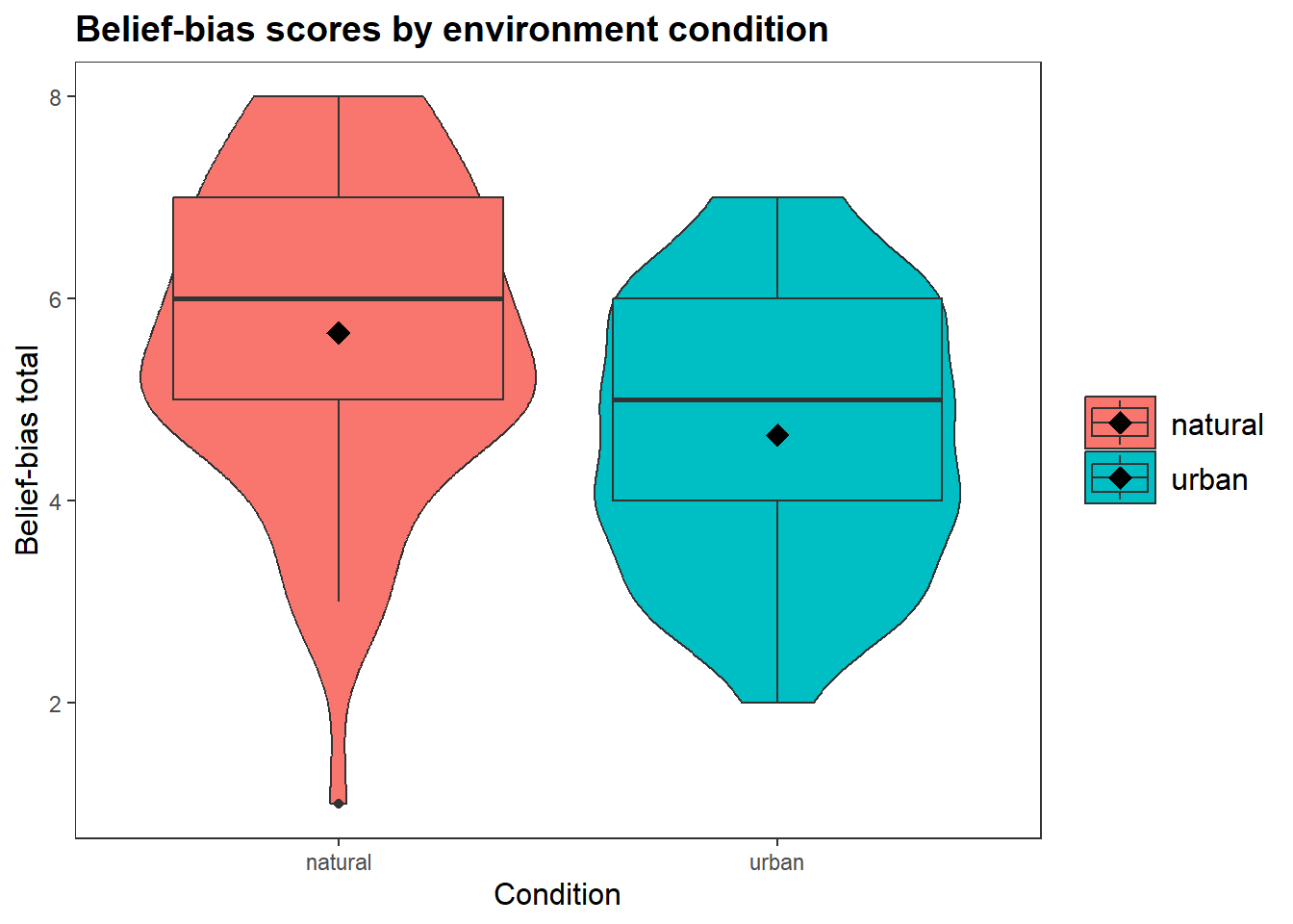

t.test(belief_bias_total ~ condition, 
       alternative = "two.sided",
       data = df_clean)


    Welch Two Sample t-test

data:  belief_bias_total by condition
t = 4.1406, df = 130.69, p-value = 0.00006172
alternative hypothesis: true difference in means between group natural and group urban is not equal to 0
95 percent confidence interval:
 0.5275799 1.4929192
sample estimates:
mean in group natural   mean in group urban 
             5.661765              4.651515

Winning rule

The fastest correct team wins.

A dataset is only correct if it has:

the correct rows
the correct columns
the correct values